This tutorial package embeds tools to download and load datasets. They can be imported from nilearn.datasets:
>>> from nilearn import datasets
>>> haxby_files = datasets.fetch_haxby_simple()
>>> # The structures contains paths to haxby dataset files:
>>> haxby_files.keys()
['data', 'session_target', 'mask', 'conditions_target']
>>> import nibabel
>>> haxby_data = nibabel.load(haxby_files.func)
>>> haxby_data.get_data().shape # 1452 time points and a spatial size of 40x64x64
(40, 64, 64, 1452)
| fetch_haxby([data_dir, n_subjects, url, ...]) | Download and loads complete haxby dataset |
| fetch_haxby_simple([data_dir, url, resume, ...]) | Download and load an example haxby dataset |
| fetch_nyu_rest([n_subjects, sessions, ...]) | Download and loads the NYU resting-state test-retest dataset. |
| fetch_adhd([n_subjects, data_dir, url, ...]) | Download and load the ADHD resting-state dataset. |
The data are downloaded only once and stored locally, in one of the following directories (in order of priority):
- the folder specified by data_dir parameter in the fetching function if it is specified
- the environment variable NILEARN_DATA if it exists
- the nilearn_data folder in the current directory
Note that you can copy that folder across computers to avoid downloading the data twice.
NIfTI and Analyse file structures
NifTi files (or Analyze files) are the standard way of sharing data in neuroimaging. We may be interested in the following three main components:
| data: | raw scans bundled in a numpy array: data = img.get_data() |
|---|---|
| affine: | gives the correspondance between voxel index and spatial location: affine = img.get_affine() |
| header: | informations about the data (slice duration...): header = img.get_header() |
Neuroimaging data can be loaded simply thanks to nibabel. Once the file is downloaded, a single line is needed to load it.
from nilearn import datasets
haxby_files = datasets.fetch_haxby_simple()

# Get the file names relative to this dataset
bold = haxby_files.func

# Load the NIfTI data
import nibabel
nifti_img = nibabel.load(bold)
fmri_data = nifti_img.get_data()
fmri_affine = nifti_img.get_affine()
Dataset formatting: data shape
We can find two main representations for MRI scans:
Niimg: Niimg (pronounce ni-image) is a common term used in Nilearn. A Niimg-like object can either be:
- a file path to a Nifti or Analyse image
- any object exposing get_data() and get_affine() methods, for instance a Nifti1Image from nibabel.
Niimg-4D: Similarly, some functions require 4-dimensional Nifti-like data, which we call Niimgs, or Niimg-4D. Accepted inputs are then:
- A path to a 4-dimensional Nifti image
- List of paths to 3-dimensional Nifti images
- 4-dimensional Nifti-like object
- List of 3-dimensional Nifti-like objects
Note
Image affines
If you provide a sequence of Nifti images, all of them must have the same affine.
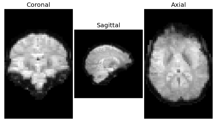
Once that NIfTI data are loaded, visualization is simply the display of the desired slice (the first three dimensions) at a desired time point (fourth dimension). For haxby, data is rotated so we have to turn each image counter-clockwise.
import numpy as np
import pylab as pl

# Compute the mean EPI: we do the mean along the axis 3, which is time
mean_img = np.mean(fmri_data, axis=3)

# pl.figure() creates a new figure
pl.figure(figsize=(7, 4))

# First subplot: coronal view
# subplot: 1 line, 3 columns and use the first subplot
pl.subplot(1, 3, 1)
# Turn off the axes, we don't need it
pl.axis('off')
# We use pl.imshow to display an image, and use a 'gray' colormap
# we also use np.rot90 to rotate the image
pl.imshow(np.rot90(mean_img[:, 32, :]), interpolation='nearest',
          cmap=pl.cm.gray)
pl.title('Coronal')

# Second subplot: sagittal view
pl.subplot(1, 3, 2)
pl.axis('off')
pl.title('Sagittal')
pl.imshow(np.rot90(mean_img[15, :, :]), interpolation='nearest',
          cmap=pl.cm.gray)

# Third subplot: axial view
pl.subplot(1, 3, 3)
pl.axis('off')
pl.title('Axial')
pl.imshow(np.rot90(mean_img[:, :, 32]), interpolation='nearest',
          cmap=pl.cm.gray)
pl.subplots_adjust(left=.02, bottom=.02, right=.98, top=.95,
                   hspace=.02, wspace=.02)
If we do not have a mask of the relevant regions available, a brain mask can be easily extracted from the fMRI data using the nilearn.masking.compute_epi_mask function:
| compute_epi_mask(epi_img[, lower_cutoff, ...]) | Compute a brain mask from fMRI data in 3D or 4D ndarrays. |
# Simple computation of a mask from the fMRI data
from nilearn.masking import compute_epi_mask
mask_img = compute_epi_mask(nifti_img)
mask_data = mask_img.get_data().astype(bool)

# We create a new figure
pl.figure(figsize=(3, 4))
# A plot the axial view of the mask to compare with the axial
# view of the raw data displayed previously
pl.axis('off')
pl.imshow(np.rot90(mask_data[:, :, 32]), interpolation='nearest')
pl.subplots_adjust(left=.02, bottom=.02, right=.98, top=.95)

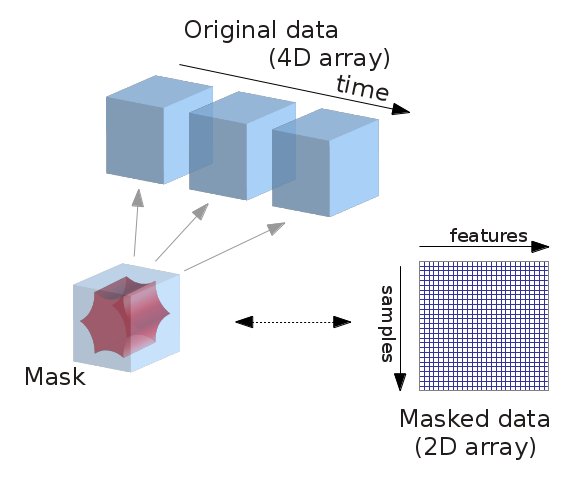
fMRI data is usually represented as a 4D block of data: 3 spatial dimensions and one of time. In practice, we are most often only interested in working only on the time-series of the voxels in the brain. It is thus convenient to apply a brain mask and go from a 4D array to a 2D array, voxel x time, as depicted below:
from nilearn.masking import apply_mask
masked_data = apply_mask(nifti_img, mask_img)
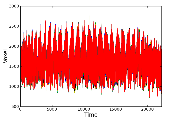
# masked_data shape is (instant number, voxel number). We can plot the first 10
# lines: they correspond to timeseries of 10 voxels on the side of the
# brain
pl.figure(figsize=(7, 5))
pl.plot(masked_data[:10].T)
pl.xlabel('Time', fontsize=16)
pl.ylabel('Voxel', fontsize=16)
pl.xlim(0, 22200)
pl.subplots_adjust(bottom=.12, top=.95, right=.95, left=.12)
pl.show()
The NiftiMasker automatically calls some preprocessing functions that are available if you want to set up your own preprocessing procedure: