Before applying some complex machine learning algorithm, or perform sophisticated analysis, the first step is to read data from file and do some basic transformation on them. Nilearn offers several ways to do this. This part is concerned with only high-level classes (in modules nilearn.input_data), the description of low-level functions can be found in the reference documentation.
The philosophy underlying these classes is similar to scikit-learn‘s transformers. Objects are initialized with some parameters proper to the transformation (unrelated to the data), then the fit() method should be called, possibly specifying some data-related information (such as number of images to process), to perform some initial computation (e.g. fitting a mask based on the data). Then transform() can be called, with the data as argument, to perform some computation on data themselves (e.g. extracting timeseries from images).
The following parts explain how to use this API to extract voxel or region signals from fMRI data. Advanced usage of these classes requires to tweak their parameters. However, high-level objects have been designed to perform common operations. Users who want to make some specific processing may have to call low-level functions (see e.g. nilearn.signal, nilearn.masking.)
This section describes how to use the NiftiMasker class in more details than the previous description. NiftiMasker is a powerful tool to load images and extract voxel signals in the area defined by the mask. It is designed to apply some basic preprocessing steps by default with commonly used default parameters. But it is very important to look at your data to see the effects of the preprocessings and validate them.
In addition, NiftiMasker is a scikit-learn compliant transformer so that you can directly plug it into a scikit-learn pipeline.
Sometimes, some custom preprocessing of data is necessary. In this example, we will restrict Haxby dataset (which contains 1452 frames) to 150 frames to speed up computation. To do that, we load the dataset with fetch_haxby_simple(), restrict it to 150 frames and build a brand new Nifti-like object to give it to the masker. Though it is possible, there is no need to save your data in a file to pass it to a NiftiMasker. Simply use nibabel to create a Niimg in memory:
In the basic tutorial, we showed how the masker could compute a mask automatically, and it has done a good job. But, on some datasets, the default algorithm performs poorly. This is why it is very important to always look at how your data look like.
Before exploring the subject, we define a helper function to display masks. This function will display a background (composed of a mean of epi scans) and a mask as a red layer over this background.
If a mask is not given, NiftiMasker will try to compute one. It is very important to take a look at the generated mask, to see if it is suitable for your data and adjust parameters if it is not. See the NiftiMasker documentation for a complete list of mask computation parameters.
As an example, we will now try to build a mask based on a dataset from scratch. The Haxby dataset will be used since it provides a mask that we can use as a reference.

The first step is to generate a mask with default parameters and take a look at it. As an indicator, we can, for example, compare the mask to original data.
With naked eyes, we can see that the outline of the mask is not very smooth. To make it less smooth, bypass the opening step (mask_opening=0).

Looking at the NiftiMasker object, we see two interesting parameters: lower_cutoff and upper_cutoff. The algorithm ignores dark (low) values. We can tell the algorithm to ignore high values by lowering upper cutoff. Default value is 0.9, so we try 0.8 to lower a bit the threshold and get a larger mask.
masker = NiftiMasker(mask_opening=True, mask_upper_cutoff=0.8)
masker.fit(haxby_img)
cutoff_mask = masker.mask_img_.get_data().astype(np.bool)

# Plot the mask and compare it to original

# Load mask provided by Haxby
haxby_mask = nibabel.load(haxby.mask).get_data().astype(np.bool)

pl.figure(figsize=(6, 5))
pl.subplot(1, 2, 1)
display_mask(background, haxby_mask[..., 27], 'Haxby mask')

pl.subplot(1, 2, 2)
display_mask(background, cutoff_mask[..., 27], 'Mask with cutoff')
pl.subplots_adjust(top=0.8)
pl.show()
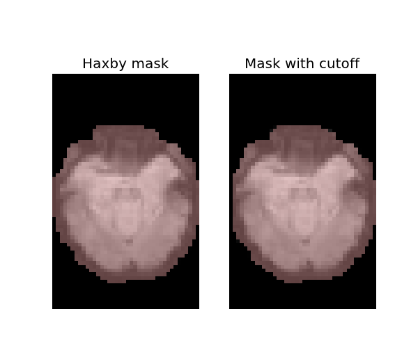
The resulting mask seems to be correct. Compared to the original one, it is very close.
Note
The full example described in this section can be found here: plot_nifti_advanced.py. This one can be relevant too: plot_nifti_simple.py.
Resampling can be used for example to reduce processing time by lowering image resolution. Certain image viewers also require images to be resampled in order to allow image fusion.
If smoothing the data prior to converting to voxel signals is required, it can be performed by NiftiMasker. It is achieved by passing the full-width half maximum (in millimeter) along each axis in the parameter smoothing_fwhm. For an isotropic filtering, passing a scalar is also possible. The underlying function handles properly the tricky case of non-cubic voxels, by scaling the given widths appropriately.
All previous filters operate on images, before conversion to voxel signals. NiftiMasker can also process voxel signals. Here are the possibilities:
Exercise
You can, more as a training than as an exercise, try to play with the parameters in plot_haxby_simple.py. Try to enable detrending and run the script: does it have a big impact on the result?
Once voxel signals have been processed, the result can be visualized as images after unmasking (turning voxel signals into a series of images, using the same mask as for masking). This step is present in almost all the examples provided in Nilearn.
The purpose of NiftiLabelsMasker and NiftiMapsMasker is to compute signals from regions containing many voxels. They make it easy to get these signals once you have an atlas or a parcellation.
Nilearn understands two different way of defining regions, which are called labels and maps, handled respectively by NiftiLabelsMasker and NiftiMapsMasker.
Note
The full example in this section can be found here: plot_adhd_covariance.py
Usage of NiftiMapsMasker and NiftiLabelsMasker is very close, and very close to the usage of NiftiMasker. Only options specific to NiftiMapsMasker and NiftiLabelsMasker are described in this section.
Nilearn provides several downloaders to get a brain parcellation. Load the MSDL one:
This atlas defines its regions using maps. The path to the corresponding file can be found under the “maps” key. Extracting region signals for several subjects can be performed like this:
region_ts is a numpy.ndarray, containing one signal per column. The subjects list contains signals for several subjects. In this example, confounds removal is performed, by both using a provided list of confounds, and by computing new ones using nilearn.image.high_variance_confounds.
One important thing that happens transparently during the execution of NiftiMasker.fit_transform is resampling. Initially, the images and the atlas do not have the same shape nor the same affine. Getting them to the same format is required for the signals extraction to work. The keyword argument resampling_target specifies which format everything should be resampled to. In the present case, “maps” indicates that all images should be resampled to have the same shape and affine as the MSDL atlas. See the reference documentation for NiftiMasker for every possible option.
The NiftiMapsMasker output can then be used as input to a scikit-learn transformer. In the present case, covariance between region signals can be obtained for each subject either using the graph lasso or the group-sparse covariance algorithm:
Usage of NiftiLabelsMasker is similar to that of NiftiMapsMasker. The main difference is that it requires a labels image instead of a set of maps as input.
The background_label keyword of NiftiLabelsMasker deserves some explanation. The voxels that correspond to the brain or a region of interest in an fMRI image do not fill the entire image. Consequently, in the labels image, there must be a label corresponding to “outside” the brain, for which no signal should be extracted. By default, this label is set to zero in Nilearn, and is referred to as “background”. Should some non-zero value occur, it is possible to change the background value with the background_label keyword.